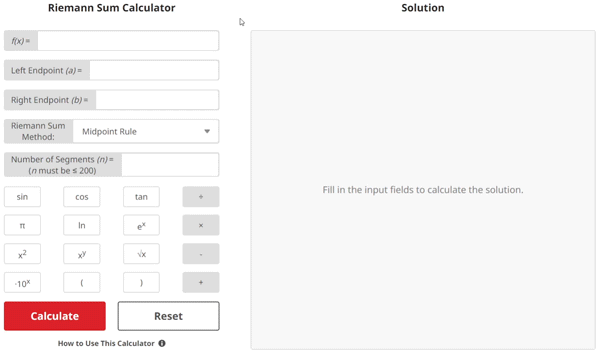
Riemann Sum Calculator
Method:
(n must be ≤ 200)
Solution


Riemann Sum Lesson
What is a Riemann Sum?
A Riemann Sum is a method that is used to approximate an integral (find the area under a curve) by fitting rectangles to the curve and summing all of the rectangles' individual areas.
In this lesson, we will discuss four summation variants including Left Riemann Sums, Right Riemann Sums, Midpoint Sums, and Trapezoidal Sums. Before we discuss the specifics of each summation variant, let's go over their similarities and the basic principles behind their functionality.
Like previously stated, a Riemann Sum is a way to approximate an integral. Well, what does this mean exactly? Let's find out:
For example, let's say that we have a parabola f(x) = x2 + 1 as seen below:
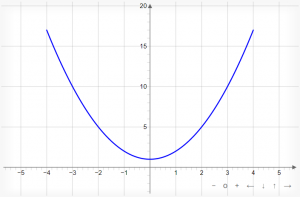
Now, if we were interested in finding the area under the curve between x = 0 and x = 4, we could either perform a definite integral as seen below...
$$\int_{0}^{4} (x^2 + 1) \text{ }dx$$
...or we can approximate this integral by:
- Choosing a certain number of equal-width rectangles (or trapezoids in the case of a trapezoidal sum) that intersect the graph from x = 0 to x = 4.
- Calculate the area of each rectangle or trapezoid.
- Add up all of the individual areas within our domain of interest (0 ≤ x ≤ 4 in this case).
Before we take a look at what this process looks like mathematically, it is important to reiterate that a Riemann Sum is an approximation. This means that there will be an inherent amount of error between the approximated area under the curve (Riemann Sum), and the actual area under the curve (definite integral). This is because the shapes that are used to intersect the graph do not perfectly fit the contours of the graphed function, resulting in parts of each shape either sticking up above the curve, or leaving gaps underneath the curve, resulting in less accurate individual area calculations. We will see specific examples of this in each summation's respective section.
Now let's see what each summation type looks like mathematically:
Why do we Learn Riemann Sums?
A Riemann Sum is useful for more than just acting as an introduction to integration. You might recall that an integration allows us to determine the area under a curve. Well, how is that relevant in real life? Let's take a look at a situation where we have a car with a faulty odometer. An odometer keeps track of the distance a car has driven in its life.
We want to know how many miles the car has driven in a single one-way trip. Since the odometer is not functioning, we can measure the vehicle's speed at fixed time intervals of equal length, then use the Riemann Sum of the data to approximate the total distance traveled in the trip of interest.
How does velocity versus time data translate to distance? When we take the integral of a velocity function versus time, we get the area under the velocity curve. This area is the net displacement (where the vehicle ended up with reference to our start point). In our example, we are looking at speed (magnitude of velocity only), which will yield the total distance traveled as the area under the curve. We can use a Riemann Sum to find this area under the curve by fitting rectangles (or trapezoids) to the data points for vehicle speed at a given time, then summing the individual areas of these shapes. The smaller the time interval between speed measurements, the more accurate of an approximation we will get for the total distance traveled.
This method doesn't even require sophisticated equipment for computation either! These calculations can be carried out using standard spreadsheet programs. Just input the recorded velocity and time data into our Riemann Sum equations, and we get an approximation of distance traveled without the need of an exact equation.
This is just one example of the many uses for this concept!
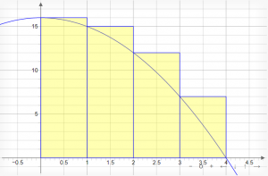
Left Riemann Sums
Here, we have a graph of the function f(x) = x2 + 1 using a Left Riemann Sum with n = 4 segments to approximate the area under the curve:
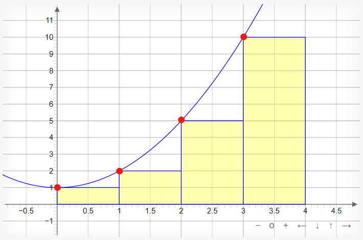
What we see here is a series of four rectangles intersecting the graph with their respective top-left corners from x = 0 to x = 4. The purpose for extending these rectangles up to the function's plotted line is so that we can find the area of each one of these rectangles and then add up all the areas so that we can approximate the area under the curve.
This can be accomplished by utilizing the equations found in the next section.
How to Calculate a Left Riemann Sum?
To calculate the Left Riemann Sum, utilize the following equations:
$$\begin{align}& \text{1.) }Area = \Delta x [f(a) + f(a + \Delta x) + f(a + 2 \Delta x) + \cdots + f(b\:-\:\Delta x)] \\ \\ & \hspace{3ex} \text{2.) } \Delta x = \frac{b-a}{n} \end{align}$$
Where Δx is the length of each subinterval (rectangle width), a is the left endpoint of the interval, b is the right endpoint of the interval, and n is the desired number of subintervals (rectangles) to be used for approximation.
This is the recommended order of operations for the above equations:
- Calculate Δx by plugging in your left endpoint a, right endpoint b, and number of desired subintervals (rectangles) n into equation 2.
- Determine where the top-left corner of each rectangle will intersect the curve by indexing your x value beginning with the left endpoint a, and then adding Δx until you get to the final x value for the last segment's top-left corner (x = b - Δx).
- Evaluate the function at each applicable x value and sum the results.
- Multiply the sum from step 3 with Δx.
NOTE: For a solved example of a Left Riemann Sum, see example problem 1.
Error When Using a Left Riemann Sum
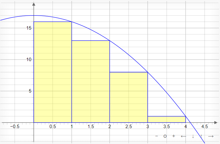
In this particular application of the Left Riemann Sum, this method will underestimate the area under the curve because there are chunks of empty space under the curve and around the rectangles that are not being added up as part of the area approximation. As a general rule of thumb, if the curve is always increasing in your interval of interest (Figure 2), a Left Riemann Sum will underestimate the area under the curve; if the curve is always decreasing in your interval of interest (Figure 3), a Left Riemann Sum will overestimate the area under the curve.
Right Riemann Sums
Here, we have a graph of function f(x) = x2 + 1 using a Right Riemann Sum with n = 4 segments to approximate the area under the curve:
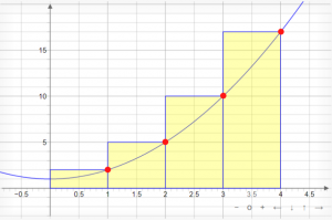
What we see here is a series of four rectangles intersecting the graph with their respective top-right corners from x = 0 to x = 4. The purpose for extending these rectangles up to the function's plotted line is so that we can find the area of each one of these rectangles and then add up all the areas so that we can approximate the area under the curve.
This can be accomplished by utilizing the equations found in the next section.
How to Calculate a Right Riemann Sum?
To calculate the Right Riemann Sum, utilize the following equations:
$$\begin{align}& \text{3.) }Area = \Delta x [f(a + \Delta x) + f(a + 2 \Delta x) + \cdots + f(b)] \\ \\ & \hspace{3ex} \text{4.) } \Delta x = \frac{b-a}{n} \end{align}$$
Where Δx is the length of each subinterval (rectangle width), a is the left endpoint of the interval, b is the right endpoint of the interval, and n is the desired number of subintervals (rectangles) to be used for approximation.
This is the recommended order of operations for the above equations:
- Calculate Δx by plugging in your left endpoint a, right endpoint b, and number of desired subintervals (rectangles) n into equation 4.
- Determine where the top-right corner of each rectangle will intersect the curve by indexing your x value beginning with x = a + Δx, and then adding Δx until you get to the final x value for the last segment's top-right corner (x = b).
- Evaluate the function at each applicable x value and sum the results.
- Multiply the sum from step 3 with Δx.
NOTE: For a solved example of a Right Riemann Sum, see example problem 2.
Error When Using a Right Riemann Sum
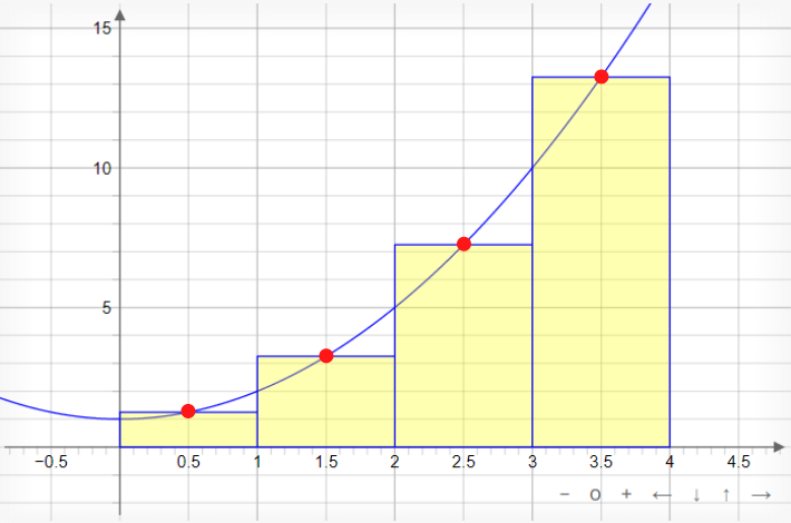
In this particular application of the Right Riemann Sum, this method will overestimate the area under the curve because there are chunks of each rectangle sticking up above the curve that are being added up as part of the area approximation. As a general rule of thumb, if the curve is always increasing in your interval of interest (Figure 4), a Right Riemann Sum will overestimate the area under the curve; if the curve is always decreasing in your interval of interest (Figure 5), a Right Riemann Sum will underestimate the area under the curve.
Midpoint Sums
Here, we have a graph of function f(x) = x2 + 1 using a Midpoint Sum with n = 4 segments to approximate the area under the curve:
What we see here is a series of four rectangles intersecting the graph with their respective midpoints from x = 0 to x = 4. The purpose for extending these rectangles up to the function's plotted line is so that we can find the area of each one of these rectangles and then add up all the areas so that we can approximate the area under the curve.
This can be accomplished by utilizing the equations in the next section.
How to Calculate a Midpoint Sum?
To calculate the Midpoint Sum, utilize the following equations:
$$\begin{align}& \text{5.) }Area = \Delta x [f(a + \frac{\Delta x}{2}) + f(a + \frac{3\Delta x}{2}) + \cdots + f(b\:-\:\frac{\Delta x}{2})] \\ \\ & \hspace{3ex} \text{6.) } \Delta x = \frac{b-a}{n} \end{align}$$
Where Δx is the length of each subinterval (rectangle width), a is the left endpoint of the interval, b is the right endpoint of the interval, and n is the desired number of subintervals (rectangles) to be used for approximation.
This is the recommended order of operations for the above equations:
- Calculate Δx by plugging in your left endpoint a, right endpoint b, and number of desired subintervals (rectangles) n into equation 6.
- Determine where the midpoint of each rectangle will intersect the curve by indexing your x value beginning with x = a + Δx/2, and then adding Δx until you get to the final x value for the last segment's midpoint (x = b - Δx/2).
- Evaluate the function at each applicable x value and sum the results.
- Multiply the sum from step 3 with Δx.
NOTE: For a solved example of a Midpoint Sum, see example problem 3.
Error When Using a Midpoint Sum
Since our rectangles intersect the curve at each respective midpoint. This yields a more accurate approximation as it does not entirely underestimate or overestimate the area under the curve. The error falls somewhere in between.
Trapezoidal Sums
Here, we have a graph of function f(x) = x2 + 1 using a Trapezoidal Sum with n = 4 segments to approximate the area under the curve:
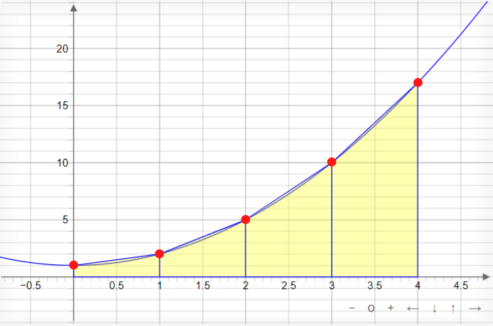
What we see here is a series of four trapezoids intersecting the graph with their respective left and right endpoints from x = 0 to x = 4. The purpose for extending these trapezoids up to the function's plotted line is so that we can find the area of each one of these trapezoids and then add up all the areas so that we can approximate the area under the curve.
This can be accomplished by utilizing the equations in the next section.
How to Calculate a Trapezoidal Sum?
To calculate the Trapezoidal Sum, utilize the following equations:
$$\begin{align}& \text{7.) }Area = \frac{1}{2}\Delta x [f(a) + 2f(a + \Delta x) + 2f(a + 2\Delta x) + \cdots + f(b)] \\ \\ & \hspace{3ex} \text{8.) } \Delta x = \frac{b-a}{n} \end{align}$$
Where Δx is the length of each subinterval (trapezoid height along x axis), a is the left endpoint of the interval, b is the right endpoint of the interval, and n is the desired number of subintervals (trapezoids) to be used for approximation.
This is the recommended order of operations for the above equations:
- Calculate Δx by plugging in your left endpoint a, right endpoint b, and number of desired subintervals (trapezoids) n into equation 8.
- Determine where the left and right endpoints of each trapezoid will intersect the curve by indexing your x value beginning with the left endpoint a and then adding Δx until you get to the final x value (right endpoint b).
- Evaluate the function at each applicable x value and sum the results.
- Multiply the sum from step 3 with Δx/2.
NOTE: For a solved example of a Trapezoidal Sum, see example problem 4.
Error When Using a Trapezoidal Sum
Since our trapezoids intersect the curve at the top-left and top-right corners of each segment, we get a closer fitment to the curve which results in a more accurate approximation of the area under the curve.
Left Riemann Sum Example Problem
$$\begin{align}& \text{1.) Using a} \textbf{ Left Riemann Sum} \text{ with 4 equal subintervals, approximate} \\ \\ & \hspace{3ex} \text{the area under the curve } f(x) \text{ = } x^2+1\text{ from } x \text{ = }0\text{ to } x \text{ = }4\\ \\ & \text{2.) For a Left Riemann Sum, the sum of the rectangles fitted to the curve} \\ \\ & \hspace{3ex} \text{(approximated area under the curve) is:} \\ \\ & \hspace{3ex} A = \Delta x \text{ } [f(a) + f(a + \Delta x) + f(a + 2 \Delta x) \hspace{1ex}+ \hspace{1ex} \cdots \hspace{1ex} + \hspace{1ex}f (b\:-\:\Delta x)]\\ \\ & \hspace{3ex} \text{Where } \Delta x = \frac{b-a}{n} \text{ is the length of each subinterval, }a \text{ is the left endpoint} \\ & \hspace{3ex} \text{of the interval, } b \text{ is the right endpoint of the interval, and } n \text{ is the desired} \\ & \hspace{3ex} \text{number of subintervals (rectangles) to be used for approximation.}\\ \\ & \text{3.) Calculate } \Delta x \text{ by inputting given values for } a, b, \text{ and } n \text{:} \\ \\ & \hspace{3ex} \Delta x = \frac{b-a}{n} \hspace{1ex} \Longrightarrow \hspace{1ex} \Delta x = \frac{4 - 0}{4} = 1\\ \\ & \text{4.) Since } \Delta x = 1, \text{our left-hand endpoints for our subintervals are:} \\ \\ & \hspace{3ex}x = 0,1,2,3\\ \\ & \text{5.) Evaluate function } f(x) = x^2+1\text{ at each of the left-hand endpoints found in} \\ & \hspace{3ex} \text{step 4:}\\ \\ & \hspace{3ex} f(0) = (0)^2+1 = 1\\ \\ & \hspace{3ex} f(1) = (1)^2+1 = 2\\ \\ & \hspace{3ex} f(2) = (2)^2+1 = 5\\ \\ & \hspace{3ex} f(3) = (3)^2+1 = 10\\ \\ & \text{6.) Input the values found in step 5 into the Left Riemann Sum equation} \\ & \hspace{3ex} \text{to approximate the area under the curve:}\\ \\ & \hspace{3ex} A = \Delta x \text{ } [f(a) + f(a + \Delta x) + f(a + 2 \Delta x) \hspace{1ex}+ \hspace{1ex} \cdots \hspace{1ex} + \hspace{1ex}f (b\: -\: \Delta x)] \\ \\ & \hspace{3ex} \Rightarrow A = (1) \text{ } [(1)+(2)+(5)+(10)] \\ \\ & \hspace{3ex} \Rightarrow A = (1)[(18)] \\ \\ & \hspace{3ex} \Rightarrow A = 18\end{align}$$
Right Riemann Sum Example Problem
$$\begin{align}& \text{1.) Using a} \textbf{ Right Riemann Sum} \text{ with 4 equal subintervals, approximate} \\ \\ & \hspace{3ex} \text{the area under the curve } f(x) \text{ = } x^2+1\text{ from } x \text{ = }0\text{ to } x \text{ = }4\\ \\ & \text{2.) For a Right Riemann Sum, the sum of the rectangles fitted to the curve} \\ \\ & \hspace{3ex} \text{(approximated area under the curve) is:} \\ \\ & \hspace{3ex} A = \Delta x \text{ } [f(a + \Delta x) + f(a + 2 \Delta x) \hspace{1ex}+ \hspace{1ex} \cdots \hspace{1ex} + \hspace{1ex}f(b)]\\ \\ & \hspace{3ex} \text{Where } \Delta x = \frac{b-a}{n} \text{ is the length of each subinterval, }a \text{ is the left endpoint} \\ & \hspace{3ex} \text{of the interval, } b \text{ is the right endpoint of the interval, and } n \text{ is the desired} \\ & \hspace{3ex} \text{number of subintervals (rectangles) to be used for approximation.}\\ \\ & \text{3.) Calculate } \Delta x \text{ by inputting given values for } a, b, \text{ and } n \text{:} \\ \\ & \hspace{3ex} \Delta x = \frac{b-a}{n} \hspace{1ex} \Longrightarrow \hspace{1ex} \Delta x = \frac{4 - 0}{4} = 1\\ \\ & \text{4.) Since } \Delta x = 1, \text{our right-hand endpoints for our subintervals are:} \\ \\ & \hspace{3ex}x = 1,2,3,4\\ \\ & \text{5.) Evaluate function } f(x) = x^2+1\text{ at each of the right-hand endpoints found in} \\ & \hspace{3ex} \text{step 4:}\\ \\ & \hspace{3ex} f(1) = (1)^2+1 = 2\\ \\ & \hspace{3ex} f(2) = (2)^2+1 = 5\\ \\ & \hspace{3ex} f(3) = (3)^2+1 = 10\\ \\ & \hspace{3ex} f(4) = (4)^2+1 = 17\\ \\ & \text{6.) Input the values found in step 5 into the Right Riemann Sum equation} \\ & \hspace{3ex} \text{to approximate the area under the curve:}\\ \\ & \hspace{3ex} A = \Delta x \text{ } [f(a + \Delta x) + f(a + 2 \Delta x) \hspace{1ex}+ \hspace{1ex} \cdots \hspace{1ex} + \hspace{1ex}f(b)] \\ \\ & \hspace{3ex} \Rightarrow A = (1) \text{ } [(2)+(5)+(10)+(17)] \\ \\ & \hspace{3ex} \Rightarrow A = (1)[(34)] \\ \\ & \hspace{3ex} \Rightarrow A = 34\end{align}$$
Midpoint Sum Example Problem
$$\begin{align}& \text{1.) Using a} \textbf{ Midpoint Riemann Sum} \text{ with 4 equal subintervals, approximate} \\ \\ & \hspace{3ex} \text{the area under the curve } f(x) \text{ = } x^2+1\text{ from } x \text{ = }0\text{ to } x \text{ = }4\\ \\ & \text{2.) For a Midpoint Riemann Sum, the sum of the rectangles fitted to the curve} \\ \\ & \hspace{3ex} \text{(approximated area under the curve) is:} \\ \\ & \hspace{3ex} A = \Delta x \text{ } [f(a + \frac{\Delta x}{2}) + f(a + \frac{3 \Delta x}{2}) \hspace{1ex}+ \hspace{1ex} \cdots \hspace{1ex} + \hspace{1ex}f (b \: - \: \frac{\Delta x}{2})]\\ \\ & \hspace{3ex} \text{Where } \Delta x = \frac{b-a}{n} \text{ is the length of each subinterval, }a \text{ is the left endpoint} \\ & \hspace{3ex} \text{of the interval, } b \text{ is the right endpoint of the interval, and } n \text{ is the desired} \\ & \hspace{3ex} \text{number of subintervals (rectangles) to be used for approximation.}\\ \\ & \text{3.) Calculate } \Delta x \text{ by inputting given values for } a, b, \text{ and } n \text{:} \\ \\ & \hspace{3ex} \Delta x = \frac{b-a}{n} \hspace{1ex} \Longrightarrow \hspace{1ex} \Delta x = \frac{4 - 0}{4} = 1\\ \\ & \text{4.) Since } \Delta x = 1, \text{our midpoints for our subintervals are:} \\ \\ & \hspace{3ex}x = 1/2,3/2,5/2,7/2\\ \\ & \text{5.) Evaluate function } f(x) = x^2+1\text{ at each of the midpoints found in} \\ & \hspace{3ex} \text{step 4:}\\ \\ & \hspace{3ex} f(0.5) = (0.5)^2+1 = 1.25\\ \\ & \hspace{3ex} f(1.5) = (1.5)^2+1 = 3.25\\ \\ & \hspace{3ex} f(2.5) = (2.5)^2+1 = 7.25\\ \\ & \hspace{3ex} f(3.5) = (3.5)^2+1 = 13.25\\ \\ & \text{6.) Input the values found in step 5 into the Midpoint Riemann Sum equation} \\ & \hspace{3ex} \text{to approximate the area under the curve:}\\ \\ & \hspace{3ex} A = \Delta x \text{ } [f(a + \frac{\Delta x}{2}) + f(a + \frac{3 \Delta x}{2}) \hspace{1ex}+ \hspace{1ex} \cdots \hspace{1ex} + \hspace{1ex}f (b \: - \: \frac{\Delta x}{2})] \\ \\ & \hspace{3ex} \Rightarrow A = (1) \text{ } [(1.25)+(3.25)+(7.25)+(13.25)] \\ \\ & \hspace{3ex} \Rightarrow A = (1)[(25)] \\ \\ & \hspace{3ex} \Rightarrow A = 25\end{align}$$
Trapezoidal Sum Example Problem
$$\begin{align}& \text{1.) Using a} \textbf{ Trapezoidal Sum} \text{ with 4 equal subintervals, approximate} \\ \\ & \hspace{3ex} \text{the area under the curve } f(x) \text{ = } x^2+1\text{ from } x \text{ = }0\text{ to } x \text{ = }4\\ \\ & \text{2.) For a Trapezoidal Sum, the sum of the trapezoids fitted to the curve} \\ \\ & \hspace{3ex} \text{(approximated area under the curve) is:} \\ \\ & \hspace{3ex} A = \frac{1}{2} \Delta x \text{ } [f(a) + 2f(a + \Delta x) + 2f(a + 2 \Delta x) \hspace{1ex}+ \hspace{1ex} \cdots \hspace{1ex} + \hspace{1ex}f (b)]\\ \\ & \hspace{3ex} \text{Where } \Delta x = \frac{b-a}{n} \text{ is the length of each subinterval, }a \text{ is the left endpoint} \\ & \hspace{3ex} \text{of the interval, } b \text{ is the right endpoint of the interval, and } n \text{ is the desired} \\ & \hspace{3ex} \text{number of subintervals (trapezoids) to be used for approximation.}\\ \\ & \text{3.) Calculate } \Delta x \text{ by inputting given values for } a, b, \text{ and } n \text{:} \\ \\ & \hspace{3ex} \Delta x = \frac{b-a}{n} \hspace{1ex} \Longrightarrow \hspace{1ex} \Delta x = \frac{4 - 0}{4} = 1\\ \\ & \text{4.) Since } \Delta x = 1, \text{our endpoints for our subintervals are:} \\ \\ & \hspace{3ex}x = 0,1,2,3,4\\ \\ & \text{5.) Evaluate function } f(x) = x^2+1\text{ at each of the endpoints found in} \\ & \hspace{3ex} \text{step 4:}\\ \\ & \hspace{3ex} f(0) = (0)^2+1 = 1\\ \\ & \hspace{3ex} f(1) = (1)^2+1 = 2\\ \\ & \hspace{3ex} f(2) = (2)^2+1 = 5\\ \\ & \hspace{3ex} f(3) = (3)^2+1 = 10\\ \\ & \hspace{3ex} f(4) = (4)^2+1 = 17\\ \\ & \text{6.) Input the values found in step 5 into the Trapezoidal Sum equation} \\ & \hspace{3ex} \text{to approximate the area under the curve:}\\ \\ & \hspace{3ex} A = \frac{1}{2} \Delta x \text{ } [f(a) + 2f(a + \Delta x) + 2f(a + 2 \Delta x) \hspace{1ex}+ \hspace{1ex} \cdots \hspace{1ex} + \hspace{1ex}f (b)] \\ \\ & \hspace{3ex} \Rightarrow A = \frac{1}{2}(1) \text{ } [(1)+(4)+(10)+(20)+(17)] \\ \\ & \hspace{3ex} \Rightarrow A = \frac{1}{2}(1)[(52)] \\ \\ & \hspace{3ex} \Rightarrow A = 26\end{align}$$
How the Calculator Works
The Riemann Sum Calculator was developed using HTML (Hypertext Markup Language), CSS (Cascading Style Sheets), and JS (JavaScript). The HTML portion of the code creates the framework of the calculator. This is what defines various entities such as the calculator space, solution box, and graph space.
CSS is then utilized for the aesthetic design of these elements. Everything from the color of the calculator keys, to the shape of the solution box is styled using CSS.
To add functionality to the calculator, JavaScript is used to allow the calculator buttons to work, perform the calculations of the user's Riemann Sums, and generate the helpful graph of the user's input function and parameters.
All of these different elements come together to produce a highly detailed and intuitive experience that helps the user understand the concepts more easily.