What is a Partial Derivative?

Suppose we have a function z = f(x,y). The output, z, is dependent on two variables: x and y. A partial derivative measures the rate of change of function z with respect to the change in either independent variable x or y. In other words, partial derivatives tell us what the change in a function is with respect to the change in one of the independent variables.

Why do we Learn About Partial Derivatives?

It is easy to think of calculus as a subject that is only useful or relevant in a classroom setting. However, calculus is used in many different ways to accomplish everything from putting a rocket into space to maximizing profits in a specific business operation.

In this case, let's take a look at how we can use partial derivatives to maximize profits as we pack and ship products to customers:

Let's say that we manage the shipping department for a company that sells a product to online customers. With the holiday season rapidly approaching, we need to balance the right amount of seasonal employees and full-time employees so that we can maximize our daily profits.

Seasonal employees cost the company less to employ since they get paid less per hour than the full-time employees and do not qualify for additional company benefits. However, the seasonal employees are typically less productive than the full-time employees due to their comparatively lower level of experience.

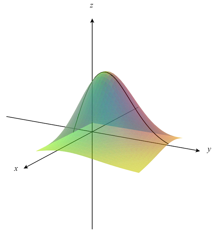
We can couple this information with historical data that relates profits to the number of seasonal and full-time employees to maximize earning potential. With enough data, the plotted points of this function would create a surface on a three dimensional graph where the z-axis represents the profits based on the independent variables x (seasonal employees) and y (full-time employees).

By using partial derivatives, we can see the change in profits with respect to the change in each type of employee. In other words, if we were to slice the three-dimensional graph along a fixed value for full-time employees (y-values), the three dimensional graph turns into a two-dimensional curve parallel to the x-z plane (see Figure 1). Taking the partial derivative of the function with respect to the number of seasonal employees effectively reveals the slope of the curve (change in profits) as the number of seasonal employees changes.

The above technique can also be used to hold the number of seasonal employees constant to see the curve parallel to the y-z plane (see Figure 2). Taking the partial derivative with respect to the number of full-time employees would then show us the slope of the curve (change in profit) as the number of full-time employees changes.

By combining this insight with the relevant computational tools and techniques, we can quickly find the maximum profit value, and in turn, the number of each employee type that correlates to this value.

The important takeaway here is the fact that we can use calculus to improve and optimize things ranging from high-level scientific applications to everyday business operations. With these tools in our mathematical toolbox, we can get the most out of our efforts.

How to Solve a Partial Differentiation Problem

If the given function has "+" or "-" signs that separate terms (ex: f(x,y) = x² + y³), the steps for solving a partial differentiation problem are as follows:

1. Break the expression into pieces by using the "+" or "-" signs as separators.
2. If computing ∂f/∂x, take the derivative of the pieces from Step 1 with respect to x while treating y as a constant. If computing ∂f/∂y, take the derivative of the pieces from Step 1 with respect to y while treating x as a constant.
3. Put the resulting pieces from Step 2 back into a single expression.
4. If you are required to evaluate the partial derivative at a point (x,y), plug the values for x and y into the result from Step 3 and simplify.

If the given function does NOT have "+" or "-" signs that separate terms (ex: f(x,y) = -x²), the steps for solving a partial differentiation problem are as follows:

1. If computing ∂f/∂x, take the derivative of the given function with respect to x while treating y as a constant. If computing ∂f/∂y, take the derivative of the given function with respect to y while treating x as a constant.
2. If you are required to evaluate the partial derivative at a point (x,y), plug the values for x and y into the result from Step 1 and simplify.

Partial Derivative Example Problem 1

$$\begin{align} & \text{Solution Steps:} \\ \\ & \hspace{3ex} \text{Compute }\frac{\partial f}{\partial x}\text{ for }f(x,y) = x^2+y-10\\ \\ & \hspace{3ex} \text{Additionally, evaluate }\frac{\partial f}{\partial x}\text{ at }(x,y) = (1, 2)\\ \\ & \hspace{3ex} \text{Let's begin by taking the partial derivative of each part of the} \\ & \hspace{3ex} \text{function with respect to }x\text{. It can be helpful for us to think of this as} \\ & \hspace{3ex} \text{the following process:} \\ \\ & \hspace{3ex} \text{1.) Break the function into pieces by using '+' or '-' signs as separators.} \\ & \hspace{3ex} \text{2.) Take the deriviative of these pieces with respect to }x\text{ while treating } \\ & \hspace{6.5ex}y\text{ as a constant.} \\ & \hspace{3ex} \text{3.) Put the resulting pieces back together into a single expression.} \\ & \hspace{3ex} \text{4.) Evaluate }\frac{\partial f}{\partial x}\text{ at }(x,y) = (1, 2).\\ \\ & \text{1.) Breaking the function } \:f(x, y) = x^2+y-10\:\text{ into pieces, we get:} \\\\ & \hspace{3ex} \text{1.}1\text{) }\;x^2\\\\ & \hspace{3ex} \text{1.}2\text{) }\;y\\\\ & \hspace{3ex} \text{1.}3\text{) }\;-10\\\\ & \text{2.) Next, let's compute } \frac{\partial f}{\partial x}\text{ for the individual pieces found in Step 1. } \\ & \hspace{3ex} \text{Variable }y\text{ will be treated as a constant:} \\\\ & \hspace{3ex} \text{2.}1\text{) }\;\frac{\partial f}{\partial x}\text{ (}x^2\text{) } = 2 \hspace{0ex} x\\\\ & \hspace{3ex} \text{2.}2\text{) }\;\frac{\partial f}{\partial x}\text{ (}y\text{) } = 0\\\\ & \hspace{3ex} \text{2.}3\text{) }\;\frac{\partial f}{\partial x}\text{ (}-10\text{) } = 0\\\\ & \text{3.) Next, let's put the individual }\frac{\partial f}{\partial x}\text{ pieces found in Step 2 back together} \\ & \hspace{3ex} \text{into a single expression:} \\ \\ & \hspace{3ex} \Longrightarrow\frac{\partial f}{\partial x} = 2 x\\ \\ & \text{4.) Now, let's plug the given values for }x \text{ and } y \text{ into the expression found} \\ & \hspace{3ex} \text{in Step 3 and evaluate.} \\ \\ & \hspace{3ex} \Longrightarrow \frac{\partial f}{\partial x} = 2 x\\ \\ & \hspace{3ex} \Longrightarrow \frac{\partial f}{\partial x}\text{ evaluated at }(1, 2) = 2 \hspace{0ex} (1)\\ \\ & \hspace{3ex} \Longrightarrow 2\\ \\ & \text{Therefore, the partial derivative of }f \text{ with respect to }x\text{ is:} \\ \\ & \Longrightarrow \boxed{\boxed{\frac{\partial f}{\partial x} = 2 x}} \\ \\ & \text{and} \\ \\ & \Longrightarrow \boxed{\boxed{\frac{\partial f}{\partial x}\text{ evaluated at (}1, 2) = 2}}\end{align}$$

Partial Derivative Example Problem 2

$$\begin{align} & \text{Solution Steps:} \\ \\ & \hspace{3ex} \text{Compute }\frac{\partial f}{\partial y}\text{ for }f(x,y) = x^2+y-10\\ \\ & \hspace{3ex} \text{Additionally, evaluate }\frac{\partial f}{\partial y}\text{ at }(x,y) = (1, 2)\\ \\ & \hspace{3ex} \text{Let's begin by taking the partial derivative of each part of the} \\ & \hspace{3ex} \text{function with respect to }y\text{. It can be helpful for us to think of this as} \\ & \hspace{3ex} \text{the following process:} \\ \\ & \hspace{3ex} \text{1.) Break the function into pieces by using '+' or '-' signs as separators.} \\ & \hspace{3ex} \text{2.) Take the deriviative of these pieces with respect to }y\text{ while treating } \\ & \hspace{6.5ex}x\text{ as a constant.} \\ & \hspace{3ex} \text{3.) Put the resulting pieces back together into a single expression.} \\ & \hspace{3ex} \text{4.) Evaluate }\frac{\partial f}{\partial y}\text{ at }(x,y) = (1, 2).\\ \\ & \text{1.) Breaking the function } \:f(x, y) = x^2+y-10\:\text{ into pieces, we get:} \\\\ & \hspace{3ex} \text{1.}1\text{) }\;x^2\\\\ & \hspace{3ex} \text{1.}2\text{) }\;y\\\\ & \hspace{3ex} \text{1.}3\text{) }\;-10\\\\ & \text{2.) Next, let's compute } \frac{\partial f}{\partial y}\text{ for the individual pieces found in Step 1. } \\ & \hspace{3ex} \text{Variable }x\text{ will be treated as a constant:} \\\\ & \hspace{3ex} \text{2.}1\text{) }\;\frac{\partial f}{\partial y}\text{ (}x^2\text{) } = 0\\\\ & \hspace{3ex} \text{2.}2\text{) }\;\frac{\partial f}{\partial y}\text{ (}y\text{) } = 1\\\\ & \hspace{3ex} \text{2.}3\text{) }\;\frac{\partial f}{\partial y}\text{ (}-10\text{) } = 0\\\\ & \text{3.) Next, let's put the individual }\frac{\partial f}{\partial y}\text{ pieces found in Step 2 back together} \\ & \hspace{3ex} \text{into a single expression:} \\ \\ & \hspace{3ex} \Longrightarrow\frac{\partial f}{\partial y} = 1\\ \\ & \text{4.) Now, let's plug the given values for }x \text{ and } y \text{ into the expression found} \\ & \hspace{3ex} \text{in Step 3 and evaluate.} \\ \\ & \hspace{3ex} \Longrightarrow \frac{\partial f}{\partial y} = 1\\ \\ & \hspace{3ex} \Longrightarrow \frac{\partial f}{\partial y}\text{ evaluated at }(1, 2) = 1\\ \\ & \hspace{3ex} \Longrightarrow 1\\ \\ & \text{Therefore, the partial derivative of }f \text{ with respect to }y\text{ is:} \\ \\ & \Longrightarrow \boxed{\boxed{\frac{\partial f}{\partial y} = 1}} \\ \\ & \text{and} \\ \\ & \Longrightarrow \boxed{\boxed{\frac{\partial f}{\partial y}\text{ evaluated at (}1, 2) = 1}}\end{align}$$

How the Calculator Works

The Partial Derivative Calculator is made up of three main components: HTML, CSS, and JavaScript.

HTML, or “HyperText Markup Language”, creates the basic framework of the calculator. This is what we use to define the input fields, buttons, and solution steps field.

CSS, or “Cascading Style Sheets”, is used to style everything from the color of the calculator, to the font size of the text on each of the calculator buttons. This is also how we specify the physical shape and dimensions of the solution field.

JS, or "JavaScript", breathes life into the calculator. While HTML and CSS allow the calculator to be physically present on the page with a particular aesthetic, JS allows the calculator to actually function by taking the user's inputs, computing the answer, and then returning the answer to the solution steps field.

All of this comes together to provide the user with an easy-to-use Partial Derivative Calculator that helps them learn and check their work quickly and effectively!