What is the Mean Value Theorem?

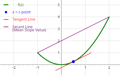
The mean value theorem tells us that a function that is continuous and differentiable between two endpoints has at least one point between the endpoints in which the tangent line of that point is parallel to the secant line through the two endpoints.

In other words, if look at the interval bound by the two endpoints, the function will always have at least one location on the interval where the value of the derivative at that location (the slope) matches the mean slope value of the function over the interval.

The formal definition of the mean value theorem for a function f(x) is given as:

• If f(x) is continuous over the closed interval [a, b]
• And if f(x) is differentiable over the open interval (a, b)
• Then there is at least one number c such that a < c < b

Where:

$$f'(c) = \frac{f(b) \; - \; f(a)}{b \; - \; a}$$

Why do we Learn About the Mean Value Theorem?

The mean value theorem is a building block for many important calculus concepts and has direct real-life applications that are often overlooked. So, let's take a quick dive into one of these overlooked real-life applications of the mean value theorem: confirming that a particle experienced a target test velocity during its trip around a particle accelerator.

Particle accelerators come in many forms, but in general, are used to accelerate very small particles to very high speeds for the sake of collecting data and learning more about how the world works.

However, it can be very hard to directly measure the velocity of a very fast, very tiny particle because we can't put a GPS (Global Positioning System) or speedometer on it. Fortunately, we can extend the concept of the mean value theorem to confirm a particle has reached a target test velocity.

If we place sensors at the beginning and end of a section of a particle accelerator and use them to detect when the particle passes each location, we will know the position and time respectively for each endpoint of the test section.

The particle's velocity will likely fluctuate as it travels over the test section due to imperfections in the accelerator's hardware. So, how do we know if the particle experienced an exact target test velocity during its pass through the section?

We can call the position our x coordinate, the time our t coordinate, and the test section our interval. Then, we can use the equation v_average = ^Δx⁄_t to determine the average velocity. This average velocity is equal to the mean slope value of the x versus t graph of our particle over the interval.

Since the mean value theorem tells us that a function must equal its mean slope value over an interval in at least one location (provided it is continuous and differentiable), we will know the particle was traveling at its calculated average velocity at least one time over the test section.

Using this data, we can adjust the propulsion power and refine further tests to make the particle experience our target test velocity. The mean value theorem gives us the power of measuring the unmeasurable!

How to use the Mean Value Theorem (Example Problem)

$$\begin{align}& \hspace{2ex} \text{Solution Steps:} \\ \\ & \hspace{2ex} \text{Determine if } f(x) \text{ meets the preliminary requirements of the mean value} \\ & \hspace{2ex} \text{theorem. If it does, find all numbers } \: x = c \: \text{ that satisfy the theorem.}\\ \\ & \hspace{2ex} \text{The mean value theorem is given as:} \\ \\ & \hspace{3ex} \bullet \text{If } f(x) \text{ is continuous over the closed interval } [a, b] \\ & \hspace{3ex} \bullet \text{And if } f(x) \text{ is differentiable over the open interval } (a, b) \\ & \hspace{3ex} \bullet \text{Then there is at least one number } \: c \: \text{ such that } \: a < c < b \\ \\ & \hspace{6ex} \text{Where } \; f'(c) = \frac{f(b) - f(a)}{b - a} \\ \\ & \hspace{6ex} \text{In other words, the slope of } f(x) \text{ at the point(s) } c \text{ is equal to} \\ & \hspace{6ex} \text{the } \textbf{average (mean) slope value} \text{ of } f(x) \text{ over the interval.}\\ \\ \\ & \hspace{2ex} \text{To solve the problem, we will:} \hspace{45ex} \\ \\ & \hspace{2ex} \text{1) Check if } f(x) \text{ is continuous over the closed interval } [a, b] \\ \\ & \hspace{2ex} \text{2) Check if } f(x) \text{ is differentiable over the open interval } (a, b) \\ \\ & \hspace{2ex} \text{3) Solve the mean value theorem equation to find all possible} \\ & \hspace{4ex} x = c \text{ values that satisfy the mean value theorem} \\ \\ & \hspace{2ex} \text{Given the inputs: } \: f(x) = x^3-2x\text{, } \: a = -2\text{, and } \: b = 4\\ \\ \\ & \hspace{2ex} \text{1) } f(x) \text{ is continuous if there are no breaks in its graph and} \\ & \hspace{4ex} \text{we would not have to pick up our pencil to draw it.} \\ \\ & \hspace{4ex} \text{Checking if } \: f(x) = x^3-2x\: \text{ is continuous over } [-2,4] \text{, we find:}\\ \\ & \hspace{4ex} \: f(x) = x^3-2x\: \text{ is fully continuous over } [-2,4]\\ \\ & \hspace{2ex} \text{2) } f(x) \text{ is differentiable if } f'(x) \text{ is continuous.} \\ & \hspace{4ex} f'(x) \text{ is continuous if there are no breaks in its graph and} \\ & \hspace{4ex} \text{we would not have to pick up our pencil to draw it.} \\ \\ & \hspace{4ex} \text{Taking the derivative of } \: f(x) = x^3-2x\text{, we get:} \\ \\ & \hspace{6ex} \Longrightarrow \; f'(x) = - 2 + 3 {x}^{2}\\ \\ & \hspace{4ex} \text{Checking if } \: f'(x) = - 2 + 3 {x}^{2}\: \text{ is continuous over } (-2,4) \text{, we find:}\\ \\ & \hspace{4ex} \: f'(x) = - 2 + 3 {x}^{2}\: \text{ is fully continuous over } (-2,4)\\ \\ & \hspace{2ex} \text{3) Now that we have determined } f(x) \text{ meets the preliminary} \\ & \hspace{4ex} \text{requirements of the mean value theorem, we will proceed} \\ & \hspace{4ex} \text{with finding all numbers } \: x = c \: \text{ that satisfy the theorem.}\\ \\ & \hspace{4ex} \text{3.1) The mean value theorem equation is given as:} \\ \\ & \hspace{8ex} f'(c) = \frac{f(b) - f(a)}{b - a} \\ \\ & \hspace{8ex} \text{Where:} \\ & \hspace{8ex} a \text{ is the interval's left endpoint } \\ & \hspace{8ex} b \text{ is the interval's right endpoint } \\ & \hspace{8ex} f(a) \text{ is } f(x) \text{ evaluated at a} \\ & \hspace{8ex} f(b) \text{ is } f(x) \text{ evaluated at b} \\ & \hspace{8ex} f'(c) \text{ is the derivative of } f(x) \text{ evaluated at c}\\ \\ & \hspace{4ex} \text{3.2) Since we already have all necessary inputs, we can plug them} \\ & \hspace{8ex} \text{into the mean value theorem equation. Doing so, we get:} \\ \\ & \hspace{10ex} \rightarrow \; a = -2 \\ & \hspace{10ex} \rightarrow \; b = 4 \\ & \hspace{10ex} \rightarrow \; f(a) = (-2)^3-2(-2) = -4 \\ & \hspace{10ex} \rightarrow \; f(b) = (4)^3-2(4) = 56 \\ & \hspace{10ex} \rightarrow \; f'(c) = - 2 + 3 {c}^{2} \\ \\ & \hspace{10ex} \Longrightarrow \; - 2 + 3 {c}^{2} = \frac{ \left( 56 \right) - \left( -4 \right) }{ \left( 4 \right) - \left( -2 \right) }\\ \\ & \hspace{4ex} \text{3.3) Simplifying the right side of the equation, we get:} \\ \\ & \hspace{10ex} \Longrightarrow \; - 2 + 3 {c}^{2} = 10\\ \\ & \hspace{4ex} \text{3.4) Now, let's solve for c. Doing so, we get:} \\ \\ & \hspace{10ex} \Longrightarrow \; c = 2,-2\\ \\ & \hspace{4ex} \text{3.5) Since } x = c = 2,-2\text{ are }\text{within our closed interval } [-2,4] \text{,} \\ & \hspace{8ex} f(x) \text{ satisfies the mean value theorem at:} \\ \\ & \hspace{10ex} \Longrightarrow \; \boxed{\boxed{ x = 2,-2}}\\ & \end{align}$$

How the Calculator Works

This calculator is created using the web programming languages HTML, CSS, and JS.

HTML (HyperText Markup Language) is the backbone of the entire system. It defines every element that we see and interact with when using the calculator. For example, the calculator buttons are HTML elements named as their respective calculator function.

CSS (Cascading Style Sheets) defines the styling and appearance of everything created by the HTML. The previously mentioned HTML calculator buttons are shaped, sized, colored, and animated by CSS code.

JS (JavaScript) makes the calculator work. When we type in a function, click a button, or have it calculate an answer, the JS code is responsible for what happens thereafter. For example, when the calculator buttons are clicked, the click is detected and written to the input field via the JS code.