What is Euler's Method?

Euler's Method is an iterative procedure for approximating the solution to an ordinary differential equation (ODE) with a given initial condition.

Euler's method is particularly useful for approximating the solution to a differential equation that we may not be able to find an exact solution for. Since this is a numerical method that uses several iterations to approach a final approximation, computers are great tools for utilizing this approach as they can carry out a large number of calculations very quickly as you may have already seen with the Euler's Method Calculator found above.

Why do we Learn Euler's Method?

We learn Euler’s method as a foundation for solving ordinary differential equations numerically. However, it is so powerful and flexible that we can also utilize it for high-level engineering feats such as the optimization of a fighter jet’s wing design.

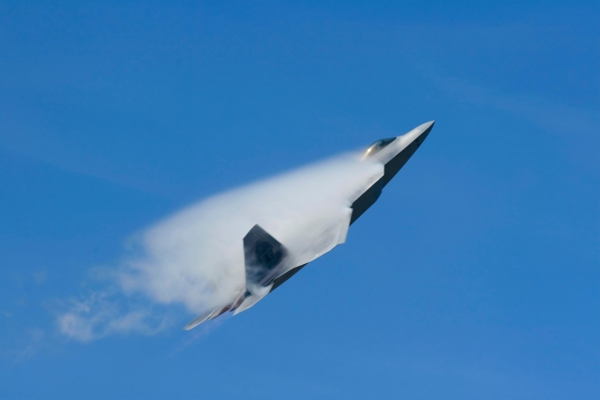
Fighter jets (like the F-22 shown above) are designed to operate across an extremely wide variety of flight conditions. Since the wings generate the massive amount of lift required for hard aerial maneuvers, we must calculate the forces that air imparts on them as the jet flies. Ideally, we will use a computer to calculate these forces for all foreseen flight conditions and tweak the wing’s design accordingly.

There is an extremely useful set of equations in engineering called the Navier–Stokes equations, which are based on the laws of conservation of momentum and conservation of mass. These equations can tell us how a fluid (air in this case) behaves as it flows. They are commonly utilized in computational fluid dynamics (CFD), which is a simulation method used by computer software that allows one to import the wing’s geometry for design optimizations.

The Navier-Stokes equations form a system of partial differential equations. However, we can reduce them down into ordinary differential equations and format Euler’s method to solve this newly created system of ordinary differential equations.

By programming this routine into a computer’s CFD software, we can input our flight condition parameters, quickly get outputs for how the wings perform under those conditions, tweak the design, and re-run the solver. When we have iterated to the point of satisfactory optimization, we will have a high-performance fighter jet wing design!

How does Euler's Method Work?

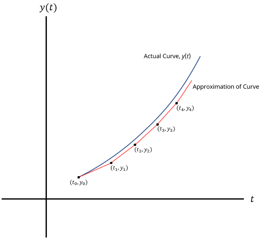
Below, we have a basic graph of some function y(t).

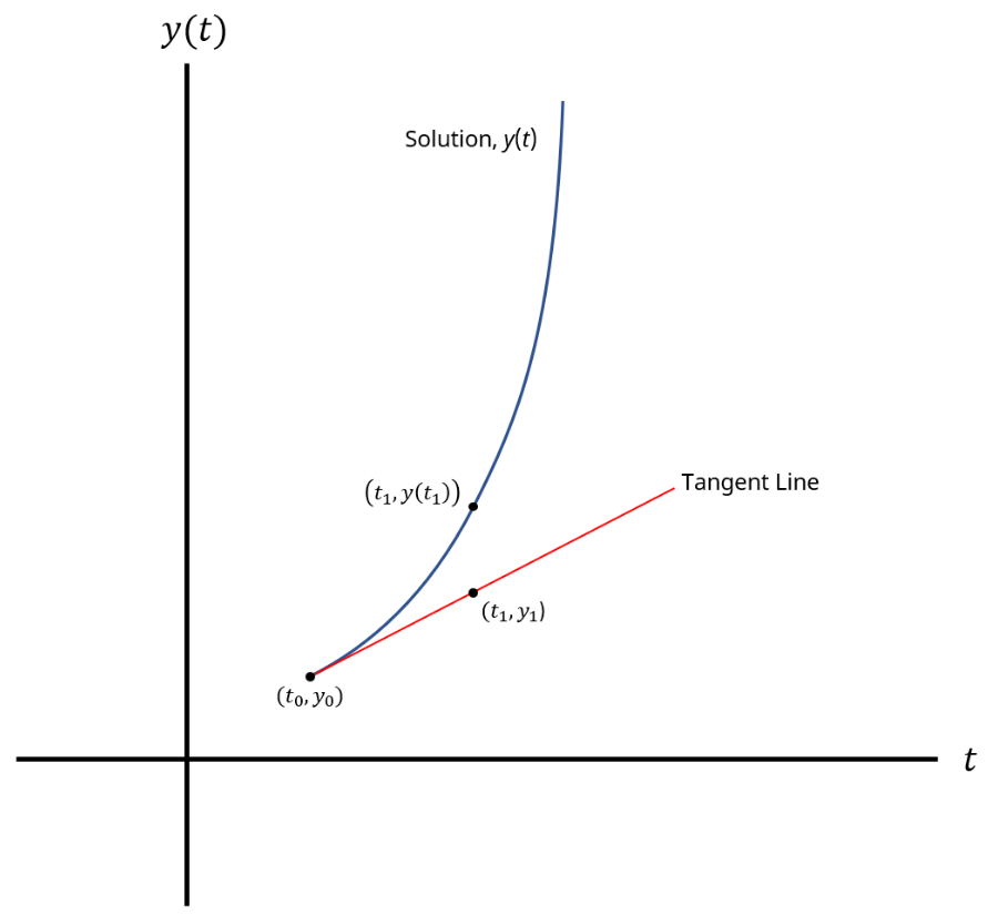
In this case, we do not know what the exact solution is. However, we can use Euler's Method to approximate the solution at a point of interest. We begin at a given a set of initial conditions in the form of an initial t value (t₀), an initial y value (y₀), and a function y' that can be identified as a function of t and y. In other words, this function y' = f (t, y).

Using this given information in conjunction with the Euler's Method equation (Equation 1), we can model a tangent line (as seen in Figure 1) that will allow us to begin approximating the solution curve. This is an iterative process where we calculate intermediate t and y values based on a specified step size (Δt) until we reach our desired end value in the form of a y value at some t value we will call t_target. In other words, we are solving for y(t_target).

Now let's take a look at the Euler's Method Equation:

$$\begin{align} & y_{i+1} = y_{i} + f (t_{i}, y_{i})\Delta t \hspace{7ex} \text{(1)} \end{align}$$

Where f (t_i, y_i) is a function of t and y that characterizes the slope of the tangent line at coordinates (t_i, y_i), t_i is the t coordinate at the current point, y_i is the y coordinate at the currrent point, and y_i+1 is the y coordinate at the next point.

Now, you might be wondering why or how the tangent line is modeled from the Euler's Method equation. To answer that, we will review the point-slope form equation (Equation 2):

$$\begin{align} & y_{1} \: - \: y_{0} = m (x_{1} \: - \: x_{0}) \hspace{7ex} \text{(2)} \end{align}$$

Where m is the slope, x₀ is the x coordinate at the first point, x₁ is the x coordinate at the second point, y₀ is the y coordinate at the first point, and y₁ is the y coordinate at the second point.

If you see the similarities between the Euler's Method equation and the point-slope form of a line, it is because Equation 1 is essentially the point-slope form equation of a line. This is what allows us to model tangent lines for the approximation of subsequent y values.

If our step size (Δt) is sufficiently small, that would mean that as we move along the tangent line from t₀ to t₁, the y value on the tangent line at t₁ is fairly close to the y value on the solution curve at t₁, making y₁ a reasonable approximation. This process is repeated until the desired target y value is reached at t_target.

Now that we have some background information on Euler's Method, let's learn how to utilize it to approximate a solution in the next section.

How to use Euler's Method to Approximate a Solution

Let's say we have the following givens:

y' = 2t + y and y(1) = 2

And we want to use Euler's Method with a step size, of Δt = 1 to approximate y(4).

To do this, we begin by recalling the equation for Euler's Method:

$$\begin{align} & y_{i+1} = y_{i} + f (t_{i}, y_{i})\Delta t\end{align}$$

Where f (t_i, y_i) is a function of t and y that characterizes the slope of the tangent line at coordinates (t_i, y_i), t_i is the t coordinate at the current point, y_i is the y coordinate at the current point, y_i+1 is the y coordinate at the next point, and Δt is the step size.

NOTE: If you are given number of steps (n) instead of step size (Δt), you can calculate the step size with Equation 3:

$$\begin{align} & \Delta t = \frac{t_{target} \: - \: t_{0}}{n} \hspace{7ex} \text{(3)}\end{align}$$

Where Δt is the step size, t_target is the t value that we are interested in using to find our target y value, t₀ is our initial t value, and n is the number of steps.

Now, let's create a basic table that we can enter our data into as we go along:

i	ti	yi
0	t0 = 1	y0 = 2
1	t1 = t0 + Δt = 2	y1 = y0 + f (t0, y0)Δt
2	t2 = t1 + Δt = 3	y2 = y1 + f (t1, y1)Δt
3	t3 = t2 + Δt = 4	y3 = y2 + f (t2, y2)Δt

The table is laid out such that the first column serves as the index for each row, the second column contains all of the t values beginning with t₀ and indexing by Δt until we reach our desired t_target value (t_target = 4 in this demonstration), and the third column is where we track our y values beginning with y₀ and ending where we get the y value that corresponds with t_target.

Let's begin adapting the Euler's Method Equation to our example and begin approximating:

As a reminder our givens were:

y' = f (t, y) = 2t + y, t₀ = 1, y₀ = 2, and Δt = 1

$$\begin{align}& \text{1.) } \text{For }i = 0: \\ \\ & \hspace{3ex} \text{1.1) Begin by substituting 0 in for } i \text{ in the Euler's Method equation.} \\ \\ & \hspace{7ex} \Rightarrow y_{(0)+1} = y_{(0)} + f(t_{(0)},y_{(0)})\Delta t \\ \\ & \hspace{7ex} \Rightarrow y_{1} = y_{0} + f(t_{0},y_{0})\Delta t \\ \\ & \hspace{3ex} \text{1.2) Now, we plug in our given values for } y_{0}, t_{0}, f(t_{0}, y_{0}), \text{ and } \Delta t \\ \\ & \hspace{7ex} \text{NOTE: In this case, } f(t_{0}, y_{0}) = 2(t_{0}) + (y_{0}) = 2(1) + (2) \\ \\ & \hspace{7ex}\Rightarrow y_{1} = (2) + (2 \cdot (1)+(2))(1) \Rightarrow y_{1} = \framebox{6} \\ \\ & \hspace{7ex} \Rightarrow \text{Therefore, } y_{1} = 6 \text{ is the approximated } y \text{ value at } t_{1} = 2\text{.} \\ & \hspace{11ex} \text{Where } t_{1} = t_{0} + \Delta t \Longrightarrow t_{1} = (1) + (1) = 2 \\ \\ & \hspace{3ex} \text{1.3) We can now update our table with our calculated }y_{1} \text{ value: } \\ \\ & \hspace{8ex} \begin{array}{ |c| |c| |c| } \hline i & t_{i} & y_{i} \\ \hline 0 & t_{0} = 1 & y_{0} = 2\\ \hline 1 & t_{1} = t_{0} + \Delta t = 2 & y_{1} = y_{0} + f(t_{0}, y_{0}) = \framebox{6} \\ \hline 2 & t_{2} = t_{1} + \Delta t = 3 & y_{2} = y_{1} + f(t_{1}, y_{1}) \\ \hline3& t_{3} = t_{2} + \Delta t = 4 & y_{3} = y_{2} + f(t_{2}, y_{2}) \\ \hline \end{array}\\ \\ & \text{2.) } \text{For }i = 1: \\ \\ & \hspace{3ex} \text{2.1) Substitute 1 in for } i \text{ in the Euler's Method equation.}\\ \\ & \hspace{7ex} \Rightarrow y_{(1)+1} = y_{(1)} + f(t_{(1)},y_{(1)})\Delta t \\ \\ & \hspace{7ex} \Rightarrow y_{2} = y_{1} + f(t_{1},y_{1})\Delta t \\ \\ & \hspace{3ex} \text{2.2) Now, we plug in our values for } y_{1}, t_{1}, f(t_{1}, y_{1}), \text{ and } \Delta t \\ \\ & \hspace{7ex} \text{NOTE: In this case, } f(t_{1}, y_{1}) = 2(t_{1}) + (y_{1}) = 2(2) + (6) \\ \\ & \hspace{7ex} \Rightarrow y_{2} = (6) + (2 \cdot (2)+(6))(1) \Rightarrow y_{2} = \framebox{16} \\ \\ & \hspace{7ex} \Rightarrow \text{Therefore, } y_{2} = 16 \text{ is the approximated } y \text{ value at } t_{2} = 3\text{.} \\ & \hspace{11ex} \text{Where } t_{2} = t_{1} + \Delta t \Longrightarrow t_{2} = (2) + (1) = 3 \\ \\ & \hspace{3ex} \text{2.3) We can now update our table with our calculated }y_{2} \text{ value: } \\ \\ & \hspace{8ex} \begin{array}{ |c| |c| |c| } \hline i & t_{i} & y_{i} \\ \hline 0 & t_{0} = 1 & y_{0} = 2\\ \hline 1 & t_{1} = t_{0} + \Delta t = 2 & y_{1} = y_{0} + f(t_{0}, y_{0}) = 6 \\ \hline 2 & t_{2} = t_{1} + \Delta t = 3 & y_{2} = y_{1} + f(t_{1}, y_{1}) = \framebox{16} \\ \hline3& t_{3} = t_{2} + \Delta t = 4 & y_{3} = y_{2} + f(t_{2}, y_{2}) \\ \hline \end{array} \\ \\ & \text{3.) } \text{For }i = 2: \\ \\ & \hspace{3ex} \text{3.1) Substitute 2 in for } i \text{ in the Euler's Method equation.} \\ \\ & \hspace{7ex} \Rightarrow y_{(2)+1} = y_{(2)} + f(t_{(2)},y_{(2)})\Delta t \\ \\ & \hspace{7ex} \Rightarrow y_{3} = y_{2} + f(t_{2},y_{2})\Delta t \\ \\ & \hspace{3ex} \text{3.2) Now, we plug in our values for } y_{2}, t_{2}, f(t_{2}, y_{2}), \text{ and } \Delta t \\ \\ & \hspace{7ex} \text{NOTE: In this case, } f(t_{2}, y_{2}) = 2(t_{2}) + (y_{2}) = 2(3) + (16) \\ \\ & \hspace{7ex} \Rightarrow y_{3} = (16) + (2 \cdot (3)+(16))(1) \Rightarrow y_{3} = \framebox{38} \\ \\ & \hspace{7ex} \Rightarrow \text{Therefore, } y_{3} = 38 \text{ is the approximated } y \text{ value at } t_{3} = 4\text{.} \\ & \hspace{11ex} \text{Where } t_{3} = t_{2} + \Delta t \Longrightarrow t_{3} = (3) + (1) = 4 \\ \\ & \hspace{3ex} \text{3.3) We can now update our table with our calculated }y_{3} \text{ value: } \\ \\ & \hspace{8ex} \begin{array}{ |c| |c| |c| } \hline i & t_{i} & y_{i} \\ \hline 0 & t_{0} = 1 & y_{0} = 2\\ \hline 1 & t_{1} = t_{0} + \Delta t = 2 & y_{1} = y_{0} + f(t_{0}, y_{0}) = 6 \\ \hline 2 & t_{2} = t_{1} + \Delta t = 3 & y_{2} = y_{1} + f(t_{1}, y_{1}) = 16 \\ \hline3& t_{3} = t_{2} + \Delta t = 4 & y_{3} = y_{2} + f(t_{2}, y_{2}) = \framebox{38} \\ \hline \end{array} \\ \\ & \hspace{3ex} \bf{Conclusion:} \\ \\ & \hspace{3ex} \text{Since } y_{3} = 38 \text{ corresponds with } t_{3} = 4 \text{ we have arrived at our desired approximation. } \\ & \hspace{3ex} \text{In other words, we were asked to find the } y \text{ value where } t = 4 \text{; since } t_{3} = 4 \text{ and } y_3 = 38 \\ & \hspace{3ex} \text{are in the same row of the table, 38 is the } y \text{ value approximation at } t = 4 \text{.}\end{align}$$

Example Problem

$$\begin{align}& \text{Solution Steps:} \hspace{10ex}\\ \\ & \text{1.) Given: } y' = \:t+y \: \text{ and } \: \: y \text{(}1\text{)} = 2\\ \\ & \hspace{3ex} \text{Use Euler's Method }\text{with }3\text{ equal steps } (n)\text{ to approximate } y(4). \hspace{20ex}\\ \\ & \text{2.) The general formula for Euler's Method is given as:} \\ \\ & \hspace{3ex} y_{i+1} = y_{i} + f(t_{i},y_{i})\Delta t \\ \\ & \hspace{3ex} \text{Where } y_{i+1} \text{ is the approximated } y \text{ value at the newest iteration, } y_{i} \text{ is the } \\ & \hspace{3ex} \text{approximated } y \text{ value at the previous iteration, } f(t_{i},y_{i}) \text{ is the given } \\ & \hspace{3ex} y \text{' function evaluated at } t_{i} \text{ and } y_{i} \text{ (} t \text{ and } y \text{ value from previous iteration),} \\ & \hspace{3ex} \text{and } \Delta t \text{ is the step size.}\\ \\ & \text{3.) The formula for the step size (} \Delta t \text{) is given as:} \\ \\ & \hspace{3ex} \Delta t = \frac{t_{target} - t_{0}}{n} \\ \\ & \hspace{3ex} \text{Where } t_{target} \text{ is the t value of interest where we want to find our} \\ & \hspace{3ex} \text{approximated } y \text{ value, } t_{0} \text{ is the initial t value given as part of the initial} \\ & \hspace{3ex} \text{conditions, and } n \text{ is the number of steps taken from } t_{0} \text{ to } t_{target} \text{.}\\ \\ & \text{4.) }\text{Since we are given the required number of steps } n = 3\text{ rather than the} \\ & \hspace{3ex} \text{step size (} \Delta t \text{), we begin by solving for } \Delta t \text{.} \\ \\ & \hspace{3ex} \Delta t = \frac{t_{target} - t_{0}}{n} \: \Longrightarrow \: \Delta t = \frac{(4) - (1)}{(3)} = 1\\ \\ & \text{5.) We can now generate a table of } t \text{ values to aid us in approximating} \\ & \hspace{3ex} y(t_{target}) = y(4) \\ \\ & \hspace{3ex}\begin{array}{ |c| |c| |c| } \hline i & t_{i} & y_{i} \\ \hline 0 & t_{0} = \boxed{1}& y_{0} = 2\\ \hline 1 & t_{1} = t_{0} + \Delta t = \boxed{2}& y_{1} = y_{0} + f(t_{0}, y_{0}) \\ \hline 2 & t_{2} = t_{1} + \Delta t = \boxed{3}& y_{2} = y_{1} + f(t_{1}, y_{1}) \\ \hline3& t_{3} = t_{2} + \Delta t = \boxed{4}& y_{3} = y_{2} + f(t_{2}, y_{2}) \\ \hline \end{array}\\ \\ & \text{6.) Using the general formula for Euler's Method, we can begin iterating} \\ & \hspace{3ex} \text{towards our final approximation.} \\ \\ & \hspace{3ex} \text{General formula: } \: y_{i+1} = y_{i} + f(t_{i},y_{i})\Delta t \\ \\ & \hspace{3ex} \text{Given: } y' = f(t,y) = \:t+y, \: \: t_{0} = 1, \: y_{0} = 2, \: \Delta t = 1\text{ (See Step 4)}\\ \\ & \text{7.) } \text{For }i = 0: \\ \\ & \hspace{3ex} \Rightarrow y_{(0)+1} = y_{(0)} + f(t_{(0)},y_{(0)})\Delta t \\ \\ & \hspace{3ex} \Rightarrow y_{1} = y_{0} + f(t_{0},y_{0})\Delta t \\ \\ & \hspace{3ex} \Rightarrow y_{1} = (2) + ((1) + (2))(1) \; \Rightarrow \; y_{1} = \boxed{5} \\ \\ & \hspace{3ex} \Rightarrow \text{Therefore, } y_{1} = 5 \text{ is the approximated } y \text{ value at } t_{1} = 2\text{.} \\ & \hspace{7ex} \text{Where } t_{1} = t_{0} + \Delta t \; \Longrightarrow \; t_{1} = (1) + (1) = 2\\ \\ & \text{8.) } \text{For }i = 1: \\ \\ & \hspace{3ex} \Rightarrow y_{(1)+1} = y_{(1)} + f(t_{(1)},y_{(1)})\Delta t \\ \\ & \hspace{3ex} \Rightarrow y_{2} = y_{1} + f(t_{1},y_{1})\Delta t \\ \\ & \hspace{3ex} \Rightarrow y_{2} = (5) + ((2) + (5))(1) \; \Rightarrow \; y_{2} = \boxed{12} \\ \\ & \hspace{3ex} \Rightarrow \text{Therefore, } y_{2} = 12 \text{ is the approximated } y \text{ value at } t_{2} = 3\text{.} \\ & \hspace{7ex} \text{Where } t_{2} = t_{1} + \Delta t \; \Longrightarrow \; t_{2} = (2) + (1) = 3\\ \\ & \text{9.) } \text{For }i = 2: \\ \\ & \hspace{3ex} \Rightarrow y_{(2)+1} = y_{(2)} + f(t_{(2)},y_{(2)})\Delta t \\ \\ & \hspace{3ex} \Rightarrow y_{3} = y_{2} + f(t_{2},y_{2})\Delta t \\ \\ & \hspace{3ex} \Rightarrow y_{3} = (12) + ((3) + (12))(1) \; \Rightarrow \; y_{3} = \boxed{27} \\ \\ & \hspace{3ex} \Rightarrow \text{Therefore, } y_{3} = 27 \text{ is the approximated } y \text{ value at } t_{3} = 4\text{.} \\ & \hspace{7ex} \text{Where } t_{3} = t_{2} + \Delta t \; \Longrightarrow \; t_{3} = (3) + (1) = 4\\ & \end{align}$$

How the Calculator Works

The Euler's Method Calculator was developed using HTML (Hypertext Markup Language), CSS (Cascading Style Sheets), and JS (JavaScript). The HTML portion of the code creates the framework of the calculator. This is what defines various entities such as the calculator space, solution box, and table space.

CSS is then utilized for the aesthetic design of these elements. This includes everything from the size and shape of the calculator, to the convenient scroll bars that allow the user to view all of their custom solution text without taking up any more space on the webpage than necessary.

JavaScript is used to provide functionality to the built-in calculator keys, perform the Euler's Method approximation of the user's input functions and conditions, and dynamically build the table of values that can be copied with the single click of a button. Once copied, the user can simply paste the table into a spreadsheet or text document and retain the original row and column structure from the calculator page.

All of these different elements come together to produce a highly detailed and intuitive experience that helps the user understand the concepts more easily.